Outputs
Location
By default, fitting results are saved in the Output/ directory. You can specify a different directory using the --output (or -o) option:
chemex fit -o <path> [other options]
Multi-Step Fit
If the fitting method involves multiple steps, each step generates its own output subdirectory named after the fitting step.
Output/
├── STEP1/
└── STEP2/
Multi-Group Fit
In any fitting step, if the dataset can be divided into multiple groups (each with distinct fitting parameters), ChemEx fits each group separately. Results for each group are stored in numbered subfolders within the Groups/ folder, with a combined summary available in the All/ folder for convenience.
For example, if all global parameters (e.g., pB, kex) are fixed or if a residue-specific model (e.g., 2st.rs) is used, residue-specific fits are performed and organized as follows:
Output/
└── STEP2/
    ├── All/
    └── Groups/
        ├── 10_11N/
        ├── 11_12N/
        ├── 12_13N/
Content
The output directory typically includes the following files and subdirectories:
run_info/
Records how the fit was started. run.toml contains runtime and command-line
metadata grouped into run, ChemEx, Python, command, inputs, and optional Git
sections. parameters_used.toml contains the parsed independent starting
parameters needed to restart the fit, including values and bounds. Parameters
calculated from expressions are not written separately because ChemEx
reconstructs them from the independent parameters and model. inputs/ contains
lightweight copies of the user-provided experiment, parameter, and method TOML
files. Raw experimental data files are not copied.
Parameters/
Contains results of the fitting as three files: fitted.toml, fixed.toml, and constrained.toml, which list parameters that were fitted, fixed, and constrained, respectively.
Example Files
- fitted.toml
- fixed.toml
- constrained.toml
[GLOBAL]
KEX_AB =  3.81511e+02 # ±8.90870e+00
PB     =  7.02971e-02 # ±1.14784e-03

[DW_AB]
15N =  2.00075e+00 # ±2.30817e-02
31N =  1.98968e+00 # ±1.90842e-02
Uncertainties (if calculated) are shown as comments preceded by "±", based on the covariance matrix from the Levenberg-Marquardt optimization.
[CS_A]
15N =  1.19849e+02 # (fixed)
31N =  1.26388e+02 # (fixed)
[GLOBAL]
KAB =  2.68192e+01 # ±3.06068e-01 ([KEX_AB] * [PB])
KBA =  3.54692e+02 # ±8.28245e+00 ([KEX_AB] * [PA])
Propagated uncertainties and applied constraints are provided in comments.
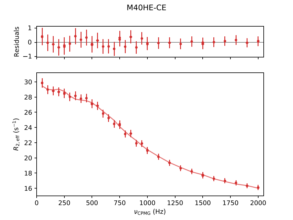
Plot/
Contains .pdf plots of the fitting results, along with the raw input and fitted data points. Example plots for CPMG and CEST experiments are shown below:
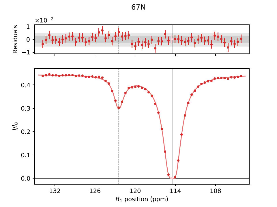
In (D-/cos-)CEST plots, solid and dashed vertical lines indicate ground and excited states, respectively, with lighter colors for filtered data points. "Folded" positions are marked with *.
Data/
Contains data values used in the fitting process along with back-calculated values for calculating χ2.
[15N]
#         NCYC   INTENSITY (EXP)       ERROR (EXP)  INTENSITY (CALC)
             0    3.47059800e+04    1.77491406e+02    3.47055362e+04
statistics.toml
Contains goodness-of-fit statistics, such as χ2.
"number of data points"                = 230
"number of variables"                  = 17
"chi-square"                           =  4.34824e+02
"reduced-chi-square"                   =  2.04143e+00
"Akaike Information Criterion (AIC)"   =  1.80479e+02
Statistics/
Contains optional uncertainty-analysis outputs requested with the STATISTICS
method-file key. Monte Carlo and bootstrap methods write summary.toml,
samples.tsv, correlations.tsv, and diagnostics.toml under
Statistics/MonteCarlo/, Statistics/Bootstrap/, and Statistics/BootstrapNS/.
MCMC writes the same file set under Statistics/MCMC/, plus a plots.pdf
report with posterior distributions, walker traces, log-probability traces, and
autocorrelation diagnostics.
The diagnostics.toml files record execution details for reproducibility. For
parallel statistics, they include the effective worker count. MCMC diagnostics
also include the direct emcee sampler engine, timing information, acceptance
fractions, burn-in decisions, and autocorrelation estimates. These diagnostics
are the best place to confirm that --workers was
applied as intended.